> For the complete documentation index, see [llms.txt](https://www.bluegamma.io/documentation/llms.txt). Markdown versions of documentation pages are available by appending `.md` to page URLs; this page is available as [Markdown](https://www.bluegamma.io/documentation/methodology/how-to-bootstrap-the-yield-curve.md).
# How We Bootstrap the Yield Curve
Learn how to bootstrap the yield curve from swap rates. Step-by-step guide to deriving zero-coupon rates and discount factors from market instruments.
BlueGamma bootstraps each interest rate curve from the latest par swap rates, with the index's latest published fixing anchoring the short end: working tenor by tenor, it solves for the discount factor that prices each swap at par, converts those discount factors into zero-coupon rates, and interpolates log-cubic on discount factors between tenors. Forward rates then follow directly from the ratio of discount factors, with no further bootstrapping.
***
## 1. Market Snapshot Philosophy
Our curves capture real market conditions at a specific timestamp:
* **Intraday updates**: for liquid markets (EUR, GBP, USD), the main curves refresh about every 30 seconds while their markets are open. See [How Often Is Your Data Refreshed?](/documentation/reference/how-often-is-your-data-refreshed.md) for other indices
* **Historical access** — Users can retrieve curves at any historical timestamp
* **Consistency** — All inputs are from the same trading session
* **Latest valid rate** — Only the most recent rate per tenor is used for curve construction
This approach aligns with how OTC derivatives and fixed income positions are typically marked for valuation.
***
## 2. Data Sources
We source data from regulated financial data vendors. The primary instruments used for curve construction are:
| Instrument | Tenors | Purpose |
| --------------------------------------------------------------- | ------------------------------------------------------------------ | -------------------------- |
| **Latest index fixing** | O/N for RFR curves; the index tenor (e.g. 6M) for term-rate curves | Anchors the short end |
| **Swaps** (OIS for RFR curves, IBOR swaps for term-rate curves) | From 1W on most OIS curves out to the longest quoted maturity | Core curve construction |
| **Fixings** | Daily | Historical reference rates |
No futures, FRAs or meeting-date swaps are used: every pillar after the fixing is a par swap quote. Swap quotes are mid, so every curve, zero rate, discount factor and forward derived from them is mid too. Quoted FRA rates are published separately through `/fras`, not used as an input, and central bank meeting probabilities are derived from the OIS curve. For the full list of indices, see [Available Indices](/documentation/data-coverage/data-coverage/available-indices.md).
***
## 3. Curve Construction Process
### Step 1: Gather Market Inputs
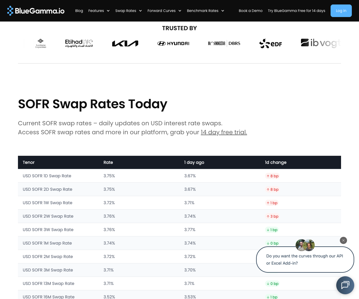
For each index, we collect the latest swap rates across all available tenors. You can see current swap rates on the [BlueGamma SOFR Swap Rates page](https://www.bluegamma.io/usd-swap-rates) or fetch them via API.
**Illustrative SOFR swap rates (December 2025 snapshot)**
| Tenor | Swap Rate |
| ----- | --------- |
| 1W | 3.72% |
| 1M | 3.75% |
| 3M | 3.71% |
| 6M | 3.63% |
| 12M | 3.47% |
| 2Y | 3.33% |
| 3Y | 3.34% |
| 5Y | 3.45% |
| 10Y | 3.78% |
| 30Y | 4.15% |
These are the **inputs** to the bootstrapping process — observable market swap rates that will be transformed into discount factors and zero-coupon rates.
### Step 2: Bootstrap the Curve
Bootstrapping the yield curve is the process of deriving zero-coupon rates and discount factors from observable market instruments. Think of it as **building a ladder** — you cannot place the 10th rung (10-year rate) until you have firmly built the 1st, 2nd, and 3rd rungs.
#### Why Bootstrap?
Zero-coupon rates aren't directly quoted by the market — they need to be derived. Bootstrapping strips away the coupon payments from swap rates to find the pure time-value of money at each maturity.
#### The Short End: Single-Payment Rates
The curve is anchored by the index's latest published fixing; every pillar after that is a swap quote. An instrument with a single payment, such as the fixing or an OIS swap of up to one year, converts straight to a discount factor:
$$
DF = \frac{1}{1 + Rate \times Time}
$$
**Example:** For illustration, take a 1-year single-payment rate of 4.00%. The discount factor is:
$$
DF\_1 = \frac{1}{1 + 0.04 \times 1.0} = 0.9615
$$
This means £1.00 received in one year is worth £0.9615 today. This becomes our **anchor point** for bootstrapping the rest of the curve.
#### The Long End: Swaps (1–30+ Years)
For longer maturities, we use **interest rate swaps**. This is where the bootstrapping algorithm becomes essential — each swap has multiple coupon payments, so we must use previously solved discount factors to isolate the unknown.
**The Key Principle:**
A par swap has zero net present value at inception. The floating leg resets to market rates, so it's worth par (the notional). Therefore, the present value of all fixed leg cash flows must also equal the notional:
$$
\sum\_{i=1}^{n} \left( Notional \times Rate \times DCF\_i \times DF\_i \right) + Notional \times DF\_n = Notional
$$
Where:
* **Notional** = Principal amount
* **Rate** = Swap rate (fixed)
* **DCF** = Day count fraction (year fraction for each period)
* **DF** = Discount factor
**The Bootstrap Loop:**
For a 2-year swap with rate 4.50%, notional £100, annual payments (DCF = 1.0):
| Year | Cash Flow | Calculation | Amount |
| ---- | --------------- | ----------------- | ------- |
| 1 | Coupon | 100 × 4.50% × 1.0 | £4.50 |
| 2 | Coupon | 100 × 4.50% × 1.0 | £4.50 |
| 2 | Notional return | 100 | £100.00 |
**Step 1: Write the par swap equation**
$$
(100 \times 0.045 \times 1.0) \times DF\_1 + (100 \times 0.045 \times 1.0 + 100) \times DF\_2 = 100
$$
Simplifying:
$$
4.50 \times DF\_1 + 104.50 \times DF\_2 = 100
$$
**Step 2: Substitute the known discount factor**
We already solved DF₁ = 0.9615 from the 1-year rate:
$$
4.50 \times 0.9615 + 104.50 \times DF\_2 = 100
$$
$$
4.327 + 104.50 \times DF\_2 = 100
$$
**Step 3: Solve for the unknown discount factor**
$$
DF\_2 = \frac{100 - 4.327}{104.50} = \frac{95.673}{104.50} = 0.9155
$$
**Step 4: Convert to zero rate**
$$
Zero\ Rate = \left(\frac{1}{DF\_2}\right)^{1/n} - 1 = \left(\frac{1}{0.9155}\right)^{1/2} - 1 = 4.51%
$$
{% hint style="info" %}
**Simplification:** The example above assumes annual payments (DCF = 1.0) and notional of 100, and quotes the zero rate with annual compounding. In practice, swaps may pay semi-annually or quarterly, and DCFs are calculated using the appropriate day count convention (e.g., Act/360, 30/360). The API's `/zero_rate` quotes simple compounding on the index day count by default; see [Zero Rates](/documentation/methodology/zero-rates.md).
{% endhint %}
#### Walking Up the Curve
For each subsequent year, we subtract the present value of **all previous coupons** before solving for the new discount factor. Here's how the curve builds up:
| Year | Instrument | Rate (Input) | Discount Factor | Zero Rate | Method |
| ---- | -------------- | ------------ | --------------- | --------- | ------------------- |
| 1 | Single payment | 4.00% | 0.9615 | 4.00% | Direct calculation |
| 2 | Swap | 4.50% | 0.9155 | 4.51% | Using Year 1 |
| 3 | Swap | 5.00% | 0.8630 | 5.03% | Using Year 1 & 2 |
| 4 | Swap | 5.25% | 0.8134 | 5.30% | Using Year 1, 2 & 3 |
Notice how the **zero rate is slightly higher than the swap rate** when the curve slopes upward. This is because swap rates are averages across the life of the swap, while zero rates represent the pure rate for that specific maturity.
{% hint style="info" %}
**Key insight:** Bootstrapping a swap curve transforms quoted swap rates (which embed coupon effects) into zero-coupon rates that can be used directly for discounting cash flows and deriving forward rates.
{% endhint %}
### Step 3: Interpolation (Connecting the Dots)
After bootstrapping, you have discount factors at specific tenors (1Y, 2Y, 3Y, etc.) — but what about 1.5 years or 6.3 years? **Interpolation** fills in the gaps.
We use **piecewise log-cubic interpolation on discount factors** to create a smooth curve between observed tenor points.
{% hint style="info" %}
**Why log discount factors?** Interpolating the logarithms of discount factors, rather than the rates themselves, keeps forward rates stable and arbitrage-free. The cubic fit keeps them smooth between pillars.
{% endhint %}
This method:
* Ensures smooth, no-arbitrage curve shapes
* Produces stable forward rates between tenor points
* Allows extraction of rates at any maturity, not just the input tenors
If log-cubic fitting fails (rare edge cases), we fall back to log-linear interpolation.
### Step 4: Extrapolation
Beyond the last quoted pillar, the curve is extrapolated from its final pillars. The longest available tenor varies by index; see [How far out do BlueGamma's curves go?](/documentation/reference/how-far-out-do-bluegammas-curves-go.md).
### Deriving the Forward Curve
Once you've bootstrapped the zero curve, deriving **forward rates** is straightforward — no additional bootstrapping required.
The zero curve tells you the cost to borrow from **today** until a future date. The forward curve tells you the implied cost to borrow from **future date A** to **future date B**.
**The breakeven logic:**
* If borrowing for 1 year costs 3%
* And borrowing for 2 years costs 4%
* The market implies Year 2 alone must cost \~5% to make the maths work
$$
Forward\_{1Y \rightarrow 2Y} = \frac{DF\_1}{DF\_2} - 1
$$
The result is a curve showing what the market expects interest rates to be at each future date — derived entirely from the discount factors you bootstrapped.
***
## 4. Multi-Curve Framework
Post-2008, the market moved to a multi-curve framework where:
* **Discounting curves** — Used for present value calculations (typically OIS-based)
* **Projection curves** — Used for forecasting floating rate cashflows (index-specific)
BlueGamma maintains separate curves for each purpose:
| Currency | Discounting Curve | Projection Curves |
| -------- | ----------------- | ---------------------- |
| USD | SOFR | SOFR |
| EUR | €STR | 1M/3M/6M EURIBOR, €STR |
| GBP | SONIA | SONIA |
| CAD | CORRA | CORRA |
For collateralised derivatives, OIS discounting is the market standard.
***
## 5. Real Example: SOFR Curve from API Data
Let's walk through a complete example using real data from the BlueGamma API: the SOFR curve on 17 December 2025.
### Input: SOFR Swap Rates
Live SOFR swap rates — the input to the bootstrapping process
**Fetch the swap curve via API:**
```bash
curl "https://api.bluegamma.io/v1/get_swap_curve?index=SOFR" \
-H "x-api-key: your_api_key"
```
The swap rates on that date are the ones shown in the Step 1 table above.
### Output: Discount Factors and Zero Rates
After bootstrapping, you can query the resulting discount factors and zero rates. Passing `valuation_time` reads them from that day's curve, so the calls below reproduce the numbers shown:
```bash
# Get the 1-year discount factor
curl "https://api.bluegamma.io/v1/discount_factor?index=SOFR&date=2026-12-17&valuation_time=2025-12-17T11:08:56" \
-H "x-api-key: your_api_key"
```
**Response:**
```json
{
"index": "SOFR",
"date": "2026-12-17",
"valuation_time": "2025-12-17T11:08:56",
"discount_factor": 0.9659,
"timestamp": "2025-12-17T11:07:56"
}
```
```bash
# Get the 1-year zero rate
curl "https://api.bluegamma.io/v1/zero_rate?index=SOFR&date=2026-12-17&valuation_time=2025-12-17T11:08:56" \
-H "x-api-key: your_api_key"
```
**Response:**
```json
{
"index": "SOFR",
"date": "2026-12-17",
"valuation_time": "2025-12-17T11:08:56",
"zero_rate": 3.477,
"day_count": "Actual360",
"compounding": "Simple",
"timestamp": "2025-12-17T11:07:56"
}
```
### Complete Bootstrapped Curve
Here's what the bootstrapping process produces for SOFR:
| Maturity | Swap Rate (Input) | Discount Factor | Zero Rate |
| ------------- | ----------------- | --------------- | --------- |
| 1Y (Dec 2026) | 3.47% | 0.9659 | 3.48% |
| 2Y (Dec 2027) | 3.33% | 0.9357 | 3.39% |
| 3Y (Dec 2028) | 3.34% | 0.9049 | 3.45% |
Notice:
* The **discount factors** decrease as maturity increases (money in the future is worth less today)
* The **zero rates** are quoted with simple compounding on Act/360, the API default. Beyond one year, a simple rate sits above the annually compounded rate for the same discount factor, which accounts for most of the gap to the swap rates here. With `compounding=Compounded`, the same discount factors give 3.48%, 3.33% and 3.34%
***
## 6. Data Quality & Validation
Reliable curves require reliable inputs. We apply multiple layers of validation to ensure the data you receive is accurate and consistent.
### Automated Checks
Every time we ingest market data, we run checks before the curve is published:
| Check | Description |
| --------------------- | ------------------------------------------------- |
| **Staleness** | Filters out rates that haven't updated recently |
| **Magnitude** | Flags unusually large moves for review |
| **Monotonicity** | Detects unexpected inversions in the long end |
| **Smoothness** | Identifies abrupt jumps between adjacent tenors |
| **Outlier detection** | Uses statistical filters to catch anomalous rates |
### Curve-Level Validation
After bootstrapping, we validate the entire curve:
| Validation | Description |
| -------------------------------- | ---------------------------------------------------- |
| **Forward rate sanity** | Forward rates should be positive and reasonable |
| **Discount factor monotonicity** | Discount factors must decrease with maturity |
| **Arbitrage-free** | No negative forward rates where they shouldn't exist |
### Human Oversight
Automation catches most issues, but human review adds an extra layer of confidence:
* **Daily curve review** — Curves are visually inspected each day by a rotating team member
* **User feedback** — Anomalies flagged by users are investigated promptly
### Third-Party Validation
We perform daily validation against public sources where available — including central bank publications, official fixing rates, and publicly available benchmark data. This ensures our curves remain aligned with observable market references.
### Validating Against Your Sources
If you want to compare BlueGamma data against Bloomberg or other platforms, see our guide: [Validating BlueGamma API Data Against Bloomberg](/documentation/reference/validating-bluegamma-api-data-against-bloomberg-or-other-platforms.md).
### Reporting Issues
If you spot something unusual, reach out via live chat in the app or email .
***
## 7. Output Conventions
| Convention | OIS Curves | IBOR Curves |
| ------------- | --------------------------------------------------------------------- | --------------------------------------------------------------------- |
| Compounding | Simple (default; Compounded or Continuous selectable on `/zero_rate`) | Simple (default; Compounded or Continuous selectable on `/zero_rate`) |
| Day Count | Act/360 (USD), Act/365 (GBP) | Index-specific |
| Business Days | Follows market calendar | Follows market calendar |
| Settlement | Index-specific (e.g. T+2 for SOFR, T+0 for SONIA) | T+2 (standard) |
***
## 8. Using Curves in BlueGamma
To pull these outputs yourself, see the API guides:
* [Fetching a Swap Curve](/documentation/integrations/api/how-to-guides/fetching-a-swap-curve.md)
* [Fetching a Swap Rate](/documentation/integrations/api/how-to-guides/fetching-a-swap-rate.md)
* [Getting Forward Rates](/documentation/integrations/api/how-to-guides/getting-forward-rates.md)
* [Getting Discount Factors](/documentation/integrations/api/how-to-guides/getting-discount-factors.md)
* [Fetching Zero Rates](/documentation/integrations/api/how-to-guides/fetching-zero-rates.md)
In Excel, the same values come from `SWAP_RATE`, `FORWARD_RATE`, `DISCOUNT_FACTOR` and `ZERO_RATE`; see [Excel Add-in Functions](/documentation/integrations/excel-add-in/functions.md).
***
## Related Documentation
* [Forward Rates](/documentation/methodology/forward-rates.md) — How forward rates are derived from curves
* [Discount Factors](/documentation/methodology/discount-factors.md) — How discount factors are calculated
* [Government Bond Curves](/documentation/methodology/government-bond-curves.md) — Treasury yield curve construction
* [Available Indices](/documentation/data-coverage/data-coverage/available-indices.md) — Full list of supported indices
* [API Reference](/documentation/integrations/api/api-reference.md) — Complete API documentation
***
## Ready to Use These Curves?
Skip the bootstrapping and get production-ready discount factors, zero rates, and forward curves directly:
| Method | Best For |
| -------------------------------------------------------------------------------------- | ---------------------------------- |
| [**Excel Add-in**](/documentation/integrations/excel-add-in/installation-and-setup.md) | Financial models, quick lookups |
| [**API**](/documentation/integrations/api/api-reference.md) | Automated systems, pricing engines |
| [**Web App**](https://app.bluegamma.io) | Ad-hoc downloads, team sharing |
[**Start your 14-day free trial →**](https://auth.bluegamma.io/sign-up)
---
# Agent Instructions
This documentation is published with GitBook. GitBook is the documentation platform designed so that both humans and AI agents can read, navigate, and reason over technical content effectively. Learn more at gitbook.com.
## Querying This Documentation
If you need additional information that is not directly available in this page, you can query the documentation by asking a question.
Perform an HTTP GET request on the following URL with the `ask` and `goal` query parameters:
```
GET https://www.bluegamma.io/documentation/methodology/how-to-bootstrap-the-yield-curve.md?ask=&goal=
```
`ask` is the immediate question: it should be specific, self-contained, and written in natural language.
`goal` is what the user is ultimately trying to achieve, the reason they need the answer. Sharing it helps GitBook give you a better, more relevant answer. A goal is most helpful when it describes the outcome the user wants rather than restating the question. For example, with `ask=how do I create an API token`, a goal like `automate deployments from our CI pipeline` lets GitBook tailor the answer to that use case.
The response will contain a direct answer to the question and relevant excerpts and sources from the documentation.
Use this mechanism when the answer is not explicitly present in the current page, you need clarification or additional context, or you want to retrieve related documentation sections.