EURIBOR API: Complete Guide to the BlueGamma API for EURIBOR

This comprehensive guide shows you everything you can do with the BlueGamma API for EURIBOR, from calculating live swap rates to building complete forward curves for derivatives pricing.

To follow along with the EURIBOR API tutorial, request API access by filling out this form or by talking to our sales team via the chat.

Check our full API Documentation here.

BlueGamma’s API provides access to all three EURIBOR tenors:

• 1M EURIBOR - One-month Euro Interbank Offered Rate
• 3M EURIBOR - Three-month Euro Interbank Offered Rate
• 6M EURIBOR - Six-month Euro Interbank Offered Rate

We also offer access to a huge range of other interest rates.

The API enables you to:

• Calculate EURIBOR swap rates for any maturity
• Build complete forward curves for derivatives pricing
• Retrieve discount factors for present value calculations
• Access historical swap rate data for backtesting and analysis

Getting Started with the EURIBOR API

Prerequisites

First, you’ll need:

• A BlueGamma API key (sign up here)
• Python 3.7 or higher
• The requests and matplotlib libraries

Install the required library:

pip install requests
pip install matplotlib

Basic Setup

Create a simple Python script to set up your API connection:

import requests
import json
from datetime import datetime, timedelta

# Your BlueGamma API key
API_KEY = "your_api_key_here"
BASE_URL = "https://api.bluegamma.io/v1"

# Headers for all requests
headers = {
    "x-api-key": API_KEY
}

def make_request(endpoint, params=None):
    """Helper function to make API requests"""
    url = f"{BASE_URL}/{endpoint}"
    response = requests.get(url, headers=headers, params=params)

    if response.status_code == 200:
        return response.json()
    else:
        print(f"Error {response.status_code}: {response.text}")
        return None

Understanding Live vs. Historical Data (Valuation Time)

Before requesting data, it is important to understand how to switch between live market data and historical snapshots using the valuation_time parameter.

1. Calculating Single EURIBOR Swap Rates

Interest rate swaps are crucial for hedging and speculation. The BlueGamma API calculates fair swap rates based on current market conditions. Here’s how to calculate a 5-year EURIBOR swap rate:

def get_euribor_swap_rate(index="3M EURIBOR", start_date="2D", maturity_date="5Y"):
    """
    Calculate EURIBOR swap rate

    Args:
        index: EURIBOR tenor (1M, 3M, or 6M EURIBOR)
        start_date: Start date as date string or tenor (e.g., "2D" for spot)
        maturity_date: Maturity as date string or tenor (e.g., "5Y")
    """
    endpoint = "swap_rate"
    params = {
        "index": index,
        "start_date": start_date,
        "maturity_date": maturity_date,
        "fixed_leg_frequency": "1Y"  # Annual fixed payments (standard for EUR swaps)
    }

    data = make_request(endpoint, params)

    if data:
        print(f"Index: {data['index']}")
        print(f"Start Date: {data['start_date']}")
        print(f"Maturity Date: {data['maturity_date']}")
        print(f"Swap Rate: {data['swap_rate']:.4f}%")

    return data

# Example: Calculate 5-year 3M EURIBOR swap rate
swap_5y = get_euribor_swap_rate("3M EURIBOR", "2D", "5Y")

Calculating EURIBOR Swap Rates API Output

Index: 3M EURIBOR
Start Date: 2025-11-20
Maturity Date: 2030-11-20
Swap Rate: 2.3092%

2. Retrieving a Complete Swap Curve

Instead of calculating rates one by one, you can retrieve the entire term structure using the get_swap_curve endpoint. This is more efficient and ensures all points are consistent with the same market snapshot.

def get_euribor_swap_curve(index="3M EURIBOR"):
    """Retrieve the full swap curve term structure"""

    # Note: The endpoint for the full curve is 'get_swap_curve'
    endpoint = "get_swap_curve"
    params = {
        "index": index,
        "start_date": "2D" # Spot start
    }

    data = make_request(endpoint, params)

    if data:
        # Use the variable 'index' passed to the function
        print(f"Swap Curve for {index}")

        # Valuation date usually returned, but handle missing key gracefully
        val_date = data.get('valuation_date') or data.get('valuation_time') or "N/A"
        print(f"Valuation Date: {val_date}")
        print("-" * 40)

        # Retrieve the list of points (trying common keys 'curve_points', 'curve' or 'swap_rates')
        points = data.get('curve_points') or data.get('curve') or data.get('swap_rates') or []

        if not points:
             print(f"No points found. Data keys: {list(data.keys())}")

        for point in points:
             # Check if 'tenor' or 'maturity' is the key
             t = point.get('tenor') or point.get('maturity')
             r = point.get('swap_rate') or point.get('rate')
             if t and r:
                 print(f"{t}: {r:.4f}%")

    return data

# Get the full swap curve
curve_data = get_euribor_swap_curve("3M EURIBOR")

Swap Curve API Output

Swap Curve for 3M EURIBOR
Valuation Date: 2025-11-20T12:10:42.390472
----------------------------------------
6M: 2.0577%
9M: 2.0592%
1Y: 2.0612%
15M: 2.0617%
18M: 2.0599%
21M: 2.0774%
2Y: 2.0991%
3Y: 2.1883%
4Y: 2.2792%
5Y: 2.3638%
6Y: 2.4416%
7Y: 2.5172%
8Y: 2.5894%
9Y: 2.6580%
10Y: 2.7225%
11Y: 2.7815%
12Y: 2.8355%
13Y: 2.8840%
14Y: 2.9265%
15Y: 2.9620%
16Y: 2.9905%
17Y: 3.0142%
18Y: 3.0333%
19Y: 3.0484%
20Y: 3.0605%
25Y: 3.0857%
30Y: 3.0874%
35Y: 3.0799%
40Y: 3.0674%
50Y: 3.0175%

Plot the EURIBOR Swap Curve

import matplotlib.pyplot as plt

def plot_swap_curve(curve_data, index_name="EURIBOR"):
    """Plot EURIBOR swap rate curve from get_swap_curve endpoint"""
    # Retrieve points using the same logic as above
    points = curve_data.get('curve_points') or curve_data.get('curve') or curve_data.get('swap_rates')

    if not points:
        print("No data to plot")
        return

    tenors = [p.get('tenor') or p.get('maturity') for p in points]
    rates = [p.get('swap_rate') or p.get('rate') for p in points]

    plt.figure(figsize=(12, 6))
    plt.plot(tenors, rates, marker='o', linewidth=2, markersize=8)
    plt.xlabel('Maturity')
    plt.ylabel('Swap Rate (%)')
    plt.title(f"EURIBOR Swap Rate Curve ({index_name})")
    plt.grid(True, alpha=0.3)
    plt.xticks(rotation=45)
    plt.tight_layout()
    plt.show()

# Plot the swap curve
plot_swap_curve(curve_data, "3M EURIBOR")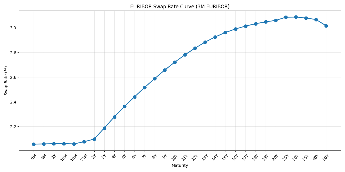

3. Building EURIBOR Forward Curves

Forward curves show expected future interest rates and are essential for pricing interest rate derivatives. Here’s how to build a complete 3M EURIBOR forward curve:

def build_euribor_forward_curve(
    index="3M EURIBOR",
    start_date=None,
    end_date=None,
    frequency="6M",
    tenor="3M"
):
    """
    Build a EURIBOR forward curve

    Args:
        index: EURIBOR tenor to use as the floating rate
        start_date: Curve start date (defaults to spot)
        end_date: Curve end date (defaults to 30 years)
        frequency: Frequency of curve points (e.g., "3M", "6M", "1Y")
        tenor: Tenor for each forward rate calculation
    """
    if start_date is None:
        start_date = (datetime.now() + timedelta(days=2)).strftime("%Y-%m-%d")

    if end_date is None:
        end_date = (datetime.now() + timedelta(days=30*365)).strftime("%Y-%m-%d")

    endpoint = "forward_curve"
    params = {
        "index": index,
        "start_date": start_date,
        "end_date": end_date,
        "frequency": frequency,
        "tenor": tenor
    }

    data = make_request(endpoint, params)

    if data:
        print(f"Forward Curve for {data.get('index', index)}")
        print(f"Period: {data.get('start_date')} to {data.get('end_date')}")
        print(f"\nForward Rates (First 5 points):")
        print("-" * 60)

        # Access the curve data
        curve = data.get('curve', [])

        for point in curve[:5]:
            print(f"{point['start_date']} to {point['end_date']}: {point['forward_rate']:.4f}%")

    return data

# Build a 30-year forward curve with semi-annual points
forward_curve = build_euribor_forward_curve(
    index="3M EURIBOR",
    frequency="6M",
    tenor="3M"
)

EURIBOR Forward Curve API Output

Forward Curve for 3M EURIBOR
Period: 2025-11-22 to 2055-11-13

Forward Rates (First 5 points):
------------------------------------------------------------
2025-11-24 to 2025-12-31: 2.0733%
2025-12-31 to 2026-03-31: 2.0472%
2026-06-30 to 2026-09-30: 1.9934%
2026-12-31 to 2027-03-31: 2.0343%
2027-06-30 to 2027-09-30: 2.1377%

Visualising the Forward Curve

Once you have the forward curve data, you can visualise the term structure of interest rates using matplotlib. This is helpful for identifying market expectations of rate hikes or cuts.

import matplotlib.pyplot as plt
from datetime import datetime

def plot_forward_curve(forward_curve_data):
    """Plot EURIBOR forward curve"""
    # Helper to check keys
    curve = forward_curve_data.get('curve', [])
    if not curve:
        return

    # Extract dates and rates from the API response
    dates = [datetime.strptime(p['start_date'], '%Y-%m-%d')
             for p in curve]
    rates = [p['forward_rate'] for p in curve]

    index_name = forward_curve_data.get('index', 'EURIBOR')

    plt.figure(figsize=(12, 6))
    plt.plot(dates, rates, marker='.', linestyle='-', linewidth=1.5)
    plt.xlabel('Date')
    plt.ylabel('Forward Rate (%)')
    plt.title(f"{index_name} Forward Curve")
    plt.grid(True, alpha=0.3)
    plt.xticks(rotation=45)
    plt.tight_layout()
    plt.show()

# Plot the forward curve calculated above
plot_forward_curve(forward_curve)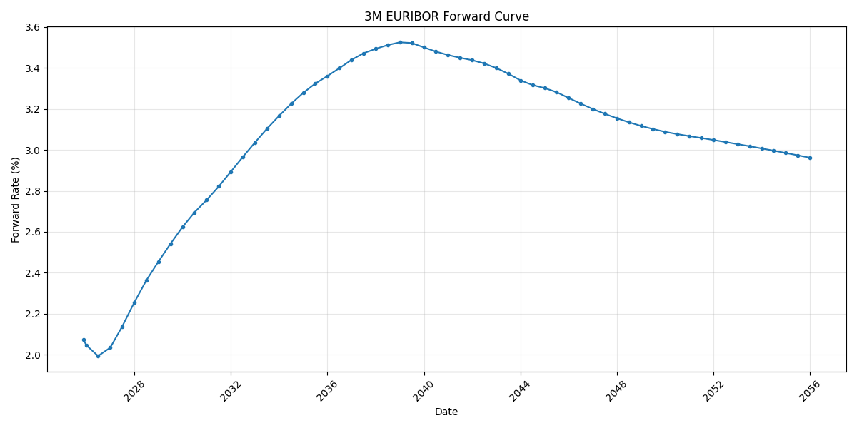

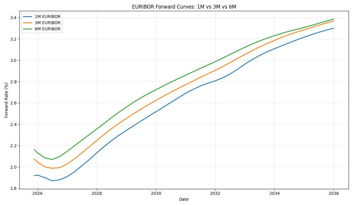
3.1 Comparing EURIBOR forward curve Tenors (Basis Spreads)

Analysing the spread between different EURIBOR tenors (1M, 3M, and 6M) is critical for understanding credit risk and liquidity preferences in the interbank market.

The following script pulls forward curves for all three tenors and plots them together to visualise the basis spreads.

def compare_euribor_curves():
    """Fetch and plot 1M, 3M, and 6M EURIBOR forward curves"""

    # Map Indices to their underlying Tenor codes
    indices = {
        "1M EURIBOR": "1M",
        "3M EURIBOR": "3M",
        "6M EURIBOR": "6M"
    }

    # Common parameters for comparison
    start_date = (datetime.now() + timedelta(days=2)).strftime("%Y-%m-%d")
    end_date = (datetime.now() + timedelta(days=10*365)).strftime("%Y-%m-%d") # 10 Year view

    plt.figure(figsize=(12, 7))

    for index_name, tenor_code in indices.items():
        params = {
            "index": index_name,
            "start_date": start_date,
            "end_date": end_date,
            "frequency": "3M", # Standardize frequency for plotting
            "tenor": tenor_code
        }

        data = make_request("forward_curve", params)

        if data and 'curve' in data:
            dates = [datetime.strptime(p['start_date'], '%Y-%m-%d') for p in data['curve']]
            rates = [p['forward_rate'] for p in data['curve']]
            plt.plot(dates, rates, label=index_name, linewidth=2)

    plt.xlabel('Date')
    plt.ylabel('Forward Rate (%)')
    plt.title('EURIBOR Forward Curves: 1M vs 3M vs 6M')
    plt.legend()
    plt.grid(True, alpha=0.3)
    plt.tight_layout()
    plt.show()

# Run the comparison
compare_euribor_curves()

What this Chart Shows

When you plot these three curves against each other, you will typically observe the following dynamics:

1. Hierarchy of Rates (Credit Risk): Under normal market conditions, 6M EURIBOR > 3M EURIBOR > 1M EURIBOR. This is because lending money for a longer period (6 months vs 1 month) carries higher credit risk and requires a liquidity premium. The gap between these lines represents the Basis Spread.
2. Spread Widening vs. Tightening:
   • Parallel Lines: Indicates stable market expectations regarding interbank credit risk.
   • Widening Spread: Often signals market stress; banks demand a higher premium to lend for longer tenors (e.g., 6M) compared to short tenors.
   • Tightening Spread: Indicates ample liquidity and low perceived credit risk in the banking sector.

4. Getting EURIBOR Discount Factors

Discount factors are crucial for calculating present values. Here’s how to retrieve them:

def get_euribor_discount_factor(index="3M EURIBOR", date=None):
    """
    Get discount factor for present value calculations

    Args:
        index: EURIBOR tenor for the curve
        date: Target date for discount factor
    """
    if date is None:
        date = (datetime.now() + timedelta(days=365)).strftime("%Y-%m-%d")

    endpoint = "discount_factor"
    params = {
        "index": index,
        "date": date
    }

    data = make_request(endpoint, params)

    if data:
        print(f"Discount Factor for {data.get('index', index)}")
        print(f"Date: {data.get('date')}")
        print(f"Discount Factor: {data.get('discount_factor'):.6f}")

    return data

# Get discount factor for 1 year from now
df_1y = get_euribor_discount_factor("3M EURIBOR")

EURIBOR Discount Factors API Output

Discount Factor for 3M EURIBOR
Date: 2026-11-20
Discount Factor: 0.979787

5. Accessing Historical Swap Rate Data

You can access historical data directly through the API to analyse trends or backtest strategies.

def get_historical_swap_rates(
    index="3M EURIBOR",
    tenor="5Y",
    start_date=None,
    end_date=None
):
    """
    Fetch historical swap rates from the API

    Args:
        index: EURIBOR tenor
        tenor: Swap maturity tenor
        start_date: Start of historical period
        end_date: End of historical period
    """
    if start_date is None:
        start_date = (datetime.now() - timedelta(days=365)).strftime("%Y-%m-%d")

    if end_date is None:
        end_date = datetime.now().strftime("%Y-%m-%d")

    endpoint = "historical_swap_rates"
    params = {
        "index": index,
        "tenor": tenor,
        "start_date": start_date,
        "end_date": end_date
    }

    data = make_request(endpoint, params)

    if data:
        print(f"Historical {index} Swap Rates")
        print(f"Tenor: {data.get('tenor', tenor)}")

        # Check structure for list of rates (handle keys 'swap_rates' or 'history')
        rates_list = data.get('swap_rates') or data.get('history') or []
        print(f"Observations: {len(rates_list)}")
        print("-" * 40)

        # Print last 10 observations
        print("Last 10 observations:")
        for obs in rates_list[-10:]:
            print(f"{obs['date']}: {obs['rate']:.4f}%")

    return data

# Retrieve historical swap rates for 5-year tenor
historical_data = get_historical_swap_rates("3M EURIBOR", "5Y")

Historical Swap Rates API Output

Historical 3M EURIBOR Swap Rates
Tenor: 5Y
Observations: 255
----------------------------------------
Last 10 observations:
2025-11-06: 2.2853%
2025-11-07: 2.2919%
2025-11-10: 2.2958%
2025-11-11: 2.2876%
2025-11-12: 2.2872%
2025-11-13: 2.3246%
2025-11-14: 2.3542%
2025-11-17: 2.3594%
2025-11-18: 2.3501%
2025-11-19: 2.3504%

Plot the historical EURIBOR Swap Rates

import matplotlib.pyplot as plt
from datetime import datetime

def plot_historical_swap_rates(history_data, index_name="3M EURIBOR"):
    """Plot historical swap rates"""
    # Handle potential key variations
    rates_list = history_data.get('swap_rates') or history_data.get('history')
    if not rates_list:
        print("No historical data found to plot")
        return

    dates = [datetime.strptime(obs['date'], '%Y-%m-%d')
             for obs in rates_list]
    rates = [obs['rate'] for obs in rates_list]

    tenor = history_data.get('tenor', '')

    plt.figure(figsize=(12, 6))
    plt.plot(dates, rates, linewidth=2)
    plt.xlabel('Date')
    plt.ylabel('Swap Rate (%)')
    plt.title(f"Historical {index_name} Swap Rates ({tenor})")
    plt.grid(True, alpha=0.3)
    plt.xticks(rotation=45)
    plt.tight_layout()
    plt.show()

# Plot the historical rates
plot_historical_swap_rates(historical_data)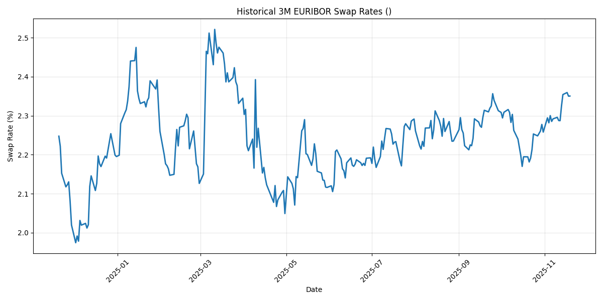

Conclusion

The BlueGamma API provides comprehensive access to everything you need for EURIBOR rate analysis. Whether you’re building a sophisticated pricing engine or just need current market rates for loan calculations, the API delivers reliable, real-time market data.

Additional Resources

• BlueGamma API Documentation
• How to Build a SOFR Forward Curve
• How to Build a CORRA Forward Curve

Need help getting started? Contact the BlueGamma team at [email protected].