What is the Zero-Coupon Yield Curve?
The Zero-Coupon Yield Curve (often called the "spot curve" or "zero curve") is a graphical representation of the yield or “spot rate” that you would earn on a single, lump-sum payment at a specific future maturity, assuming no intermediate payments.
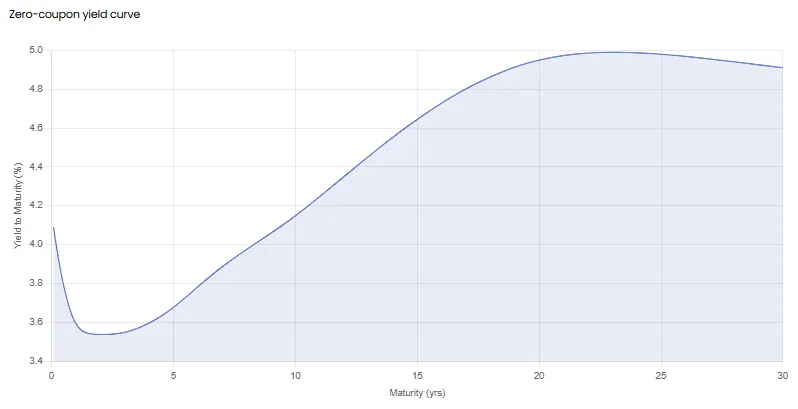
- Unlike a standard yield curve, which plots the yields of coupon-paying instruments (like standard 10-year Treasuries or Gilts), the Zero-Coupon curve represents the "pure" interest rate for a specific time horizon. It strips away the distortion caused by intermediate coupon payments, showing the true yield an investor would earn if they locked in their money today and received a single lump sum at maturity.
- While it’s rarely directly observable in the market, the curve is mathematically derived from the prices of highly liquid instruments, including government bonds and overnight index swaps. Below is a graph of a Zero-Coupon yield curve for US government bonds.
Where to access Zero-Coupon Yield Curves? We offer Zero-Coupon Bond Yield Curve data for Government Bonds and Reference Rates like SOFR, SONIA, CORRA and ESTR. No need to calculate it yourself.
You can access and embed the zero rates into your workflows in two primary ways:
- API Integration: Embed the latest zero rates directly into your treasury systems or software
- Excel Add-in: Pull real-time zero rates into your spreadsheet models using a simple, native function.
You can also access them via our Web App. Sign up for a 14-Day free Trial and navigate to the Government Bond Section of our platform to download the Zero-Coupon Bond Yield Curve of your choice.
What is the Zero-Coupon Curve used for?
The Zero-Coupon curve is the fundamental building block for modern financial valuation. Its "pure" nature makes it essential for pricing complex instruments that standard yield curves cannot handle accurately.
Its primary uses include:
- Discounting Cash Flows and Present Value Calculations:
It provides the unique discount rate required for each specific cash flow date of a security. This is required for calculating the PV of a future payment C
The discount factor D(T) is derived directly from the spot rate S(T)
This is the basis for pricing instruments like interest rate swaps, Forward Rate Agreements (FRAs), options, and structured products
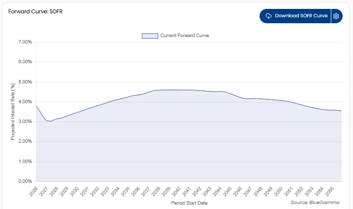
- Constructing the Forward Curve:
One of its most important applications is acting as the mathematical foundation and main component in constructing the Forward Curve, which we specialise in offering. While the Zero-Coupon curve tells you the rate for a loan starting today, the forward curve implies what the rate would be for a loan starting in the future. These are important rates used in risk management and forecasting debt service costs.
Par vs. Swap vs. Spot vs. Forward Curve
For financial modelling the word “curve” is not singular; there are several different types of curve defined by the underlying market and the choice depends on the use-case. Below we show a comparison of the different curves along with examples of BlueGamma functions, available via our Excel Add-In.
| Curve Type | Underlying Market | Practical Use Case | BlueGamma Excel Function Example |
|---|---|---|---|
| Par Curve (Government) | Government Bond Market (e.g., Treasuries, Gilts) | Country Risk (The official, sovereign risk-free rate). | - |
| Swap Curve (OIS/RFR) | Derivatives/Rates Market (e.g., SOFR, SONIA) | Pricing derivatives: Determining the fair value and fair rate of swaps. | BLUEGAMMA.DISCOUNT_RATE("SOFR", date) using overnight rates and IBORs |
| Spot Curve (Zero-Coupon) | Theoretical / Derived | Core Discount Input (The pure rate required to calculate arbitrage-free forwards and discounts). | BlueGamma.ZERO_RATE(index, date, [valuation_date]) |
| Forward Curve | Theoretical / Derived | Future Expectations (Implied rate used for forecasting and hedging future exposure). | BLUEGAMMA.FORWARD_RATE("SOFR", start_date, end_date) |
How is the Zero-Coupon Curve Constructed?
Constructing a Zero-Coupon curve is an advanced financial modelling task. Since "pure" Zero-Coupon instruments don't exist for every maturity, we must reverse-engineer the curve from coupon-bearing bonds using a method called Bootstrapping.
The basic steps are:
- Gather Data: Collect market prices for a set of liquid instruments (e.g. swaps, FRAs, futures).
- Anchor the Curve: Use short-term Zero-Coupon instruments to set the initial rates.
- Iterative Solving (Bootstrap): Move to the next longest instrument (e.g. a swap). We discount all known intermediate cash flows using the already solved rates. Then algebraically solve for the single unknown zero-rate.
- Repeat: Use the newly found rates to solve for the next maturity, stepping forward year by year until the curve is complete.
This process requires rigorous data cleaning and interpolation methods (like Cubic Spline or Nelson-Siegel) to ensure the curve is smooth and arbitrage-free.
Where can I download Zero-Coupon Bond Yield Curves?
Because Zero-Coupon yields are not directly observable for all maturities, you cannot simply "look them up" on a standard exchange; they must be calculated using the complex bootstrapping methods described above, built from market rates (like OIS, Futures and Swaps).
Most teams choose not to build these models in-house due to the risk of data errors and the maintenance required to keep the curves smooth and accurate.
You can access the Zero-Coupon curve of your choice either via our Platform, Excel add-in or API.
To gain access to our platform Sign up for a 14-Day free Trial
Zero-Coupon Yield Curve API
If you want to pull the Zero-Coupon Yield Curve via API, request API access by filling out this form or by talking to our sales team via the chat.
Here’s the API docs for our Zero Rates endpoint and an example of how to do it in Python:
pip install requests pandas matplotlib seabornimport requests
import pandas as pd
import matplotlib.pyplot as plt
import seaborn as sns
# ---------------------------------------------------------
# Configuration
# ---------------------------------------------------------
API_KEY = "YOUR-API-KEY" # Replace with your API key
BASE_URL = "https://api.bluegamma.io/v1/zero_rate"
# The specific points (tenors) we want to plot on the curve
TENORS_TO_FETCH = [
"1M", "3M", "6M", "9M",
"1Y", "2Y", "3Y", "4Y", "5Y",
"7Y", "10Y", "15Y", "20Y", "30Y"
]
def fetch_sofr_zero_curve():
"""
Loops through defined tenors and fetches the zero rate for each
using the BlueGamma /zero_rate endpoint.
"""
curve_data = []
headers = {
"x-api-key": API_KEY,
"Accept": "application/json"
}
print(f"Fetching {len(TENORS_TO_FETCH)} data points for SOFR Zero Curve...")
for tenor in TENORS_TO_FETCH:
# Parameters for the API call
params = {
"index": "SOFR",
"date": tenor, # The API accepts tenors here (e.g., "1Y")
"compounding": "Continuous", # Continuous compounding is standard for zero curves
"day_count": "Actual360" # Standard money market convention
}
try:
response = requests.get(BASE_URL, params=params, headers=headers)
if response.status_code == 200:
data = response.json()
# Store the result
curve_data.append({
"Tenor": tenor,
"Maturity Date": data['date'], # The calculated maturity date provided by API
"Zero Rate (%)": data['zero_rate'] # The rate value
})
print(f"✔ {tenor}: {data['zero_rate']}%")
else:
print(f"✖ {tenor}: Failed ({response.status_code}) - {response.text}")
except Exception as e:
print(f"Error fetching {tenor}: {e}")
return pd.DataFrame(curve_data)
def plot_curve(df):
"""
Visualizes the dataframe using Matplotlib/Seaborn
"""
if df.empty:
print("No data available to plot.")
return
# Ensure dates are datetime objects for proper sorting and plotting
df['Maturity Date'] = pd.to_datetime(df['Maturity Date'])
df = df.sort_values(by='Maturity Date')
# Setup Plot
plt.figure(figsize=(12, 6))
sns.set_style("whitegrid")
# Draw the line and the points
plt.plot(df['Maturity Date'], df['Zero Rate (%)'],
linestyle='-', linewidth=2, color="#48a8f7", label='SOFR Zero Rate (Continuous)')
# Formatting
plt.title('SOFR Zero Coupon Curve', fontsize=16, pad=15)
plt.xlabel('Maturity Date', fontsize=12)
plt.ylabel('Zero Rate (%)', fontsize=12)
plt.legend()
# Rotate x-axis dates for better readability
plt.gcf().autofmt_xdate()
plt.tight_layout()
plt.show()
if __name__ == "__main__":
# 1. Fetch Data
df = fetch_sofr_zero_curve()
# 2. Display Data Table
if not df.empty:
print("\n--- Curve Data ---")
print(df[['Tenor', 'Maturity Date', 'Zero Rate (%)']].to_string(index=False))
# 3. Plot Data
plot_curve(df)Terminal Output:
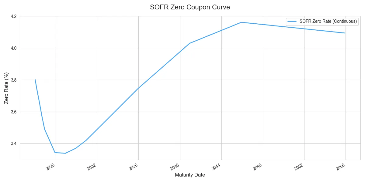
-- Curve Data ---
Tenor Maturity Date Zero Rate (%)
1M 2026-01-08 3.801107
3M 2026-03-09 3.741141
6M 2026-06-08 3.657661
9M 2026-09-08 3.568376
1Y 2026-12-08 3.489558
2Y 2027-12-08 3.344095
3Y 2028-12-08 3.339697
4Y 2029-12-10 3.372122
5Y 2030-12-09 3.422622
7Y 2032-12-08 3.551917
10Y 2035-12-10 3.747098
15Y 2040-12-10 4.031899
20Y 2045-12-08 4.163288
30Y 2055-12-08 4.095526
Zero-Coupon Curve API Visualisation:
Other derived data points
Here are some of the other derived data points you might want to access:
| Data Point | Access Method | Key Use Case & Example |
|---|---|---|
| Zero-Coupon Yield | API, App, Excel Add-in |
Retrieving the core spot rate for a specific maturity/tenor. Excel Example: =BlueGamma.ZERO_RATE(index, date, [valuation_date])
|
| Discount Factors | API, App, Excel Add-in |
Required for accurate Present Value (PV) calculations and derivatives pricing. Excel Example: =BlueGamma.DISCOUNT_RATE("SOFR", date)
|
| Forward Rates | API, App, Excel Add-in |
Essential for deriving future expected interest payments. Excel Example: =BlueGamma.FORWARD_RATE("SOFR", start_date, end_date)
|